Refreshers on some well-known models

In a general framework for inference, we observe some data $X$, which we assume to be generated by some latent variables and/or parameters $\theta$, such that we can write down a formula for $P(\mathbf{X}|\theta)$. $theta$ itself is generated from certain distribution, $P(\theta)$. Whether $\theta$ involve some latent variable or parameters, it is usually the goal of our inference to find the distribution or the values of $\theta$ given the observed data $P(\theta|X)$. Example cases of this framework are:

• In a linear regression framework: $y = X\beta + \epsilon$, where $y$ and $X$ are observed. We also assume that $\beta \sim Normal(\mathbf{0}, \sigma^2*\mathbf{I})$.
• In a Variational auto encoder, we assume that our observed data $\mathbf{X}$ of $d$ dimensions is generated, usually through a series of fully connected layers of neural networks $f$, from some latent variables $\mathbf{Z}$, i.e. $\mathbf{X} = f(\mathbf{Z})$. We may also assume that $\mathbf{Z} \sim Normal(\mathbf{0}, \sigma^2*\mathbf{I})$.
• In a Gaussian Mixture Model framework, we observe data $\mathbf{X_i}$’s. We assume that each $X_i$ may be generated from one of the $K$ Gaussian distributions, i.e. $X_i|Z_i=k \sim N(\mu_k, \Sigma_k)$. Here, $Z_i$ is the latent group-indicator variable that we want to infer, $\mu_k$ and $\Sigma_k$ are parameters that we also want to learn. There can be more layers of prior distributions for $Z_i$, $\mu_k$ and $\Sigma_k$, but the backbone of the model model is as indicated above.

Four general approaches to inference

What these models share in common is that it involves observed data $X$ and one or more layers of latent variables $\theta$. What I learned, over the years of connecting the dots (sometimes, very inefficiently, as part of my interdisciplinary training) is that we will almost will always use one of the following approaches for inference (i.e. finding $P(\theta|X)$).

• Can we write down the formula for $P(\theta|X) = \frac{P(\mathbf{X}|\theta)P(\theta)}{\int_{\theta}P(\mathbf{X}|\theta)P(\theta)d\theta}$ into a closed-form formula? If yes then do it and find the value of $\theta$ that maximizes this probability potentially through taking the derivatives $\frac{\partial P(\theta|X)}{\partial \theta}$. This is what is called Maximum A Posterori (MAP) estimation. This case usually happens when we design (assume) $P(\theta)$ to be conjugate prior to the likelihood $P(\mathbf{X}|\theta)$. If you don’t know what conjugate prior is, don’t worry, it won’t be mentioned again in this post.

• If the model is simple enough such that we can clearly break down $\theta$ to latent variables and parameters, then we can potentially use Expectation Maximization (EM) algorithm to find both the expected values of latent variables and the parameters that maximize the likelihood $P(\mathbf{X}|\theta)$ of the observed data. Usually, the first criteria for “simple enough” is that the model has only 1 layer of latent variables, i.e. $\theta \rightarrow \mathbf{X}$ and not $\theta \rightarrow \mathbf{Z} \rightarrow \cdots \rightarrow \mathbf{X}$.
• If the model is such that for each $\theta_i$ as a single latent variable/parameter in $\theta$, we can write down an analytical solution (i.e. usually, a nice known distribution PDF) for $P(\theta_i|X, \theta_{-i})$, then we can use Gibbs sampling to sequentially and repeatedly sample $\theta_i$ from $P(\theta_i|X, \theta_{-i})$ until the values of $\theta_i$’s all converge. This case, again, requires us to analytically explore the closed-form formula for $P(\theta_i|X, \theta_{-i})$ for each $\theta_i$. If you don’t know what Gibbs sampling is, don’t worry, it won’t be mentioned again in this post.
• Lastly, the most versatile approach, in my opinion, is to use Variational Inference. We will zoom into this in the following section.

Note that though the general approaches can act like recipes, our job as practitioners of the discipline is to refine these approaches based on the data at hand, hence requires the arts of implementation, trial and error. Identifying when to use which approach, unfortunately, has to be handled on a case-by-case basis. An important observation is that at each iteration, all of these approaches try to reframe the inference problem into one that can be solved by calculus, i.e. designing a loss function where the model’s latent variables and parameters $\theta$ are variables, taking derivatives, setting to $0$ and solve for $\theta$.

Variational Inference

Let’s try to understand Variational Inference (VI) and where reparameterization trick comes in through a good old example:

• Observed data: $\underbrace{\mathbf{A}}_{N \cdot D}$ and $\underbrace{\mathbf{b}}_{N \cdot 1}$. $N$: sample size, $D$: data dimension.
• Model: $\underbrace{\mathbf{A}}_{N \cdot D} \cdot \underbrace{\mathbf{\beta}}_{D \cdot 1} + \underbrace{\mathbf{\epsilon}}_{N \cdot 1} = \underbrace{\mathbf{b}}_{N \cdot 1}$, where $\mathbf{\beta} \sim Normal(\mathbf{0}, \sigma^2\cdot\mathbf{I_D})$ is the prior distribution that we assume $\mathbf{\beta}$ follows. $\mathbf{\epsilon_i} \sim Normal(\mathbf{0}, \sigma_0^2)$ is the noise term. Assume that $\sigma_0^2$ and $\sigma^2$ are known and fixed.
• Goal: Find $\mathbf{\beta}$ that fit the data, which is usually defined as the $\beta$ that maximize $P(\mathbf{\beta}| \mathbf{A}, \mathbf{b})$.

As mentioned above, there are genrally 4 approaches to this problem and in this case, it can be solved by all 4 approaches. Here, we focus on using Variational Inference (VI).

Step 1: Identifying observed data, latent variables and write down the posterior.

\(\begin{array}{|c|c|c|} \hline & \textbf{General framework} & \textbf{Example} \\ \hline Obs.data & \mathbf{X} & \mathbf{A}, \mathbf{b} \\ Latent & \mathbf{\theta} & \mathbf{\beta} \\ Prior & P(\theta) & P(\beta) = Normal(\mathbf{0}, \sigma^2\cdot\mathbf{I_D}) \\ Likelihood & P(\mathbf{X}\|\theta) & P(\mathbf{A}, \mathbf{b}\|\beta) = P(\mathbf{b}-\mathbf{A}\beta) = Normal(\mathbf{0}, \sigma_0^2) \\ Posterior & P(\mathbf{\theta}\|\mathbf{X}) & P(\beta\|\mathbf{A}, \mathbf{b})=\frac{P(\mathbf{A}, \mathbf{b}\|\beta) P{\mathbf{\beta}}}{\int_{\mathbf{\beta}} P(\mathbf{A}, \mathbf{b}\|\beta) P(\mathbf{\beta}) d\mathbf{\beta}} = Normal(\mathbf{\mu}, \mathbf{\Sigma})\\ \hline \end{array}\)
In the table above, $\mathbf{\mu}$ and $\mathbf{\Sigma}$ has a closed-form solution (due to the fact that we designed both the likelihood and the prior to be Normal). However, most of the time, in the general cases, $P(\mathbf{\theta}|\mathbf{X})$ cannot be derived analysitically. This is when I say to myself: ‘Let's try Variational Inference’.

Step 2: Write down the ELBO for the general case

If this is your first time hearing about the ELBO, just think of it as a fancy word for the loss function for variational inference, which we want to minimize. I have to rederive the ELBO for the general case each time I plan to work with variational inference, just so I can remember what to do next.

Figure 1. Derivation of the ELBO.

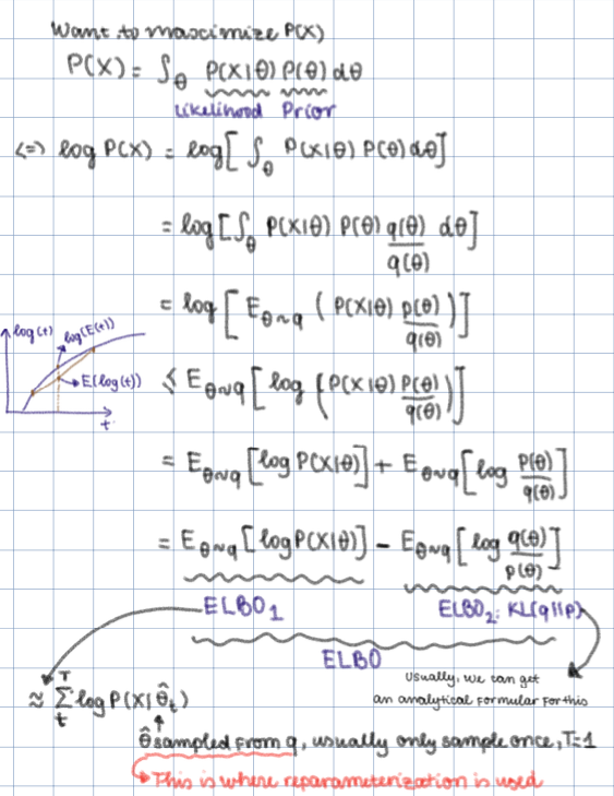
Clearly, we want to find $\theta$ that maximizes $P(X)$. What we are saying, in variational inference, is: we cannot find the exact posterior $P(\theta|\mathbf{X})$, and also cannot find the optimal $\theta$ for $P(X)$ since it is not a tractable problem. Instead, we try to generate $\theta$ from a distribution of our design $q(\theta)$ (called the variational distribution), such that we can easily sample from (i.e. some known distributions that we can easily sample by a call to functions in numpy, scipy or pytorch). The distribution $q$ has some parameters (such as mean $\mu$ for a Normal distribution) that we will optimize so that the ELBO is maximized. The ELBO, as shown above, is a lower bound for the log-likelihood $log(P(X))$.

Another amazing advantage of variational infernece is that we potentially ignore the hierarchical dependency between latent variables. If our model is such that $\theta \rightarrow \mathbf{Z} \rightarrow \cdots \rightarrow \mathbf{X}$ where besides $\mathbf{X}$, all other variables are latent and one generates another, then mean-field variational inference allows us to assume that $\theta \sim q_{\theta}$, $Z \sim q_{Z}$, etc., and $q(\text{latent vars.}) = q(\theta)\cdot q(Z) \cdots$. We just have to find the optimal parameters for each $q$ to maximize the ELBO.

Step 3: Write down the ELBO for the case at hand

In the example case, we can choose $q(\mathbf{\beta})$ to be $Normal(\underbrace{\mathbf{\mu}}_{D\cdot 1}, \mathbf{\Sigma})$, where

\(\begin{aligned} \underbrace{\mathbf{\Sigma}}_{D \cdot D}= \begin{bmatrix} \sigma_1^2 & 0 & \cdots & 0 \\ 0 & \sigma_2^2 & \cdots & 0 \\ \vdots & \vdots & \ddots & \vdots \\ 0 & 0 & \cdots & \sigma_D^2 \end{bmatrix} \end{aligned}\)
The parameters for which we will optimize for, therefore, include $\mathbf{\mu}$ and $\sigma_1^2, \sigma_2^2, \cdots, \sigma_D^2$. The ELBO for this case, based on Fig. 1, is:
\(\begin{align} \text{ELBO} &= \mathbb{E}_{q(\mathbf{\beta})} \left[ \log P(\mathbf{A}, \mathbf{b} \mid \mathbf{\beta}) \right] - KL(q(\mathbf{\beta}) \| P(\mathbf{\beta})) \\ &= \sum_{t=1}^{T} \sum_{i=1}^{N} \underbrace{\log P(\mathbf{b}_i - \mathbf{A}_i \mathbf{\beta_t})}_{N(0,\sigma_0^2)} - \underbrace{KL(q(\mathbf{\beta}) \| P(\mathbf{\beta}))}_{KL(N(\mu, \Sigma), N(\mathbf{0}, \sigma^2\cdot \mathbf{I_D}))}\\ \end{align}\)

Step 4: Reparameterize the sampled latent variables from $q$

Note that the parameters for the variational inferences include $\mu$ and $\sigma_1^2, \sigma_2^2, \cdots, \sigma_D^2$. The goal of variational inference, again, is to find the optimal values of these parameters to maximize ELBO. There usually exists an analytical fomular for $KL(q(\mathbf{\beta}) | P(\mathbf{\beta}))$ (which, in our example is the KL divergence between two MultivariateNormal distributions with different means and diagonal covariance matrices). Therefore, we can easily calculate $\frac{\partial KL(q | P)}{\partial \mu_i}$ and $\frac{\partial KL(q | P)}{\partial \sigma_i}$ for each $i \in {1,…D}$. That is one part of $\frac{\partial \text{ELBO}}{\partial \mu_i}$ and $\frac{\partial \text{ELBO}}{\partial \sigma_i}$.

However, due to the fact that we sample $\beta_t \sim N(\mu, \Sigma)$ ($t$ is index of $\beta$ samples) to construct the first part of the ELBO, we cannot easily calculate $\frac{\partial \log P(\mathbf{A}, \mathbf{b} \mid \mathbf{\beta_t}) }{\partial \mu_i}$ and $\frac{\partial \log P(\mathbf{A}, \mathbf{b} \mid \mathbf{\beta_t}) }{\partial \sigma_i}$ for each $i \in {1,…D}$. This is where the reparameterization trick comes in: Instead of directly sample $\beta_t \sim N(\mu, \Sigma)$, we sample $\epsilon_t \sim N(\mathbf{0}, \mathbf{I})$ and calculate $\beta_t = \mu + \Sigma^{1/2} \zeta_t$ where $\zeta_t \sim N(\mathbf{0}, \mathbf{I})$. This way, we can easily calculate $\frac{\partial \log P(\mathbf{A}, \mathbf{b} \mid \mathbf{\beta_t}) }{\partial \mu_i}$ and $\frac{\partial \log P(\mathbf{A}, \mathbf{b} \mid \mathbf{\beta_t}) }{\partial \sigma_i}$ because the randomness in sampling $beta_t$ got attributed to $\zeta_t$, $mu_i$ and $\sigma_i$ are included as an deterministic part of the ELBO.

Step 5: Optimize the ELBO

By this step, we have turned the problem into an optimization problem, and in turn tossing the ball into the court of optimization researchers. We, of course, need to know all the criteria for framing a solvable optimization task (such as making sure all the functions are differentiable, and the loss function should be convex if possible, etc.), but that is a topic for another post. Here, I want to provide a snapshot code for constructing the model for the example case, and the training loop.

import torch
import torch.nn as nn
import torch.optim as optim
import torch.distributions as dist
class model(nn.Module): 
    '''
    The model module specify the generative process to get to the predicted value of b given input A. 
    Required functions: __init__ and forward
    '''
    def __init__(self, D):
        super(model, self).__init__()
        self.D = D
        # set up the parameters for the variational distribution. 
        # use nn.Parameter to declare model parameters, so pytorch can keep track of the gradients
        self.mu = nn.Parameter(torch.zeros(D, 1))  # vector of mu_1, ..., mu_D
        self.sigma = nn.Parameter(torch.ones(D, 1))  # vector of sigma_1, ..., sigma_D

    @staticmethod
    def reparameterize(mu, sigma):
       eps = torch.randn_like(sigma)
       return mu + sigma * eps
    
    def forward(self, A):
        beta = self.reparameterize(self.mu, self.sigma)
        return torch.matmul(A, beta)

#### Generate data ####
N = 1000
D = 2
true_beta = torch.tensor([3, 6]).reshape(D, 1)
A = torch.randn(N, D)
b = torch.matmul(A, true_beta) + torch.randn(N, 1)

#### Loss function ####
def neg_elbo(b_pred, b, model, mu_prior=0, sigma_prior=1):
    epsilon = dist.Normal(1, 1)
    log_llh = epsilon.log_prob(b-b_pred).sum()
    model.eval()
    kl = dist.kl_divergence(dist.Normal(model.mu, model.sigma), dist.Normal(mu_prior, sigma_prior)).sum()
    return -log_llh + kl  # minimize the negative of ELBO

#### Training loop ######
model = model(D)
optimizer = optim.Adam(model.parameters(), lr=0.01)  
# the optimize registers parameters in the model for which it needs to keep track of the gradients
for epoch in range(1000):
    optimizer.zero_grad()
    b_pred = model(A)
    loss = neg_elbo(b_pred, b, model)
    loss.backward()
    optimizer.step()

#### Print the estimated beta ####
print(model.mu, model.sigma)  # model.mu can be used as the estimated beta,
# model.mu and model.sigma combined defines the estimated posterior P(beta|A, b)

Generalizing the model for other cases

So far, I have outlined the steps that I usually take when I try to apply variational inference, with an example in which the variational distribution $q$ is picked to be Normal (and hence, a reparameterization trick for normal distribution). In many cases, due to the nature of the data (categorical, continuous, non-genative, etc.), the choice of the variational distribution $q$ needs to be adapted. For example:

• In the case of Gaussian Mixture Model (presented above, first section), varitational distribution for $Z$, i.e. $q(Z_i)$ should return samples that are one-hot encoded, i.e. $Z_{i}\sim Multinomial(\pi_{q,i})$ so $Z_{i, \text{sampled}} = [0, 0, 1, 0, 0]$ for $K=5$, but the parameters for $q(Z_i)$ should be continuous, i.e. $\pi_{q,i} = [0.1, 0.2, 0.5, 0.1, 0.1]$ for $K=5$. The reparameterization trick should find a way to transform from the continuous parameters $\pi_{q,i}$ to the one-hot encoded $Z_{i, \text{sampled}}$ in a way that $\pi_{q,i}$ is still present in the ELBO. The Gumbel-Softmax trick is one way to do this (Jang, 2016).
• In my recent application, I need the latent varible to be non-negative and continuous, so I picked $q(Z_i) = LogNormal(\mu_i, \sigma_i^2)$. There is, of course, a reparameterization trick for this distribution, $Z_i = \exp(\mu_i + \sigma_i \zeta_i)$ where $\zeta_i \sim N(0, 1)$.

Conclusion

• Usually, when faced with a problem of inference, I usually try to work through four general approaches in increasing levels of problem complexity: MAP estimation, EM algorithm, Gibbs sampling, and Variational Inference.
• Variational inference is usually the most versatile approach, overcoming lots of complications in the hierarchical dependency of latent variables. If we understand the nature of the data requirements, we can pick variational distributions that are both suitable for the data, but also easy to sample from and easy to derive the KL divergence from the prior.
• I always rederive the ELBO for the general case as a separate step in my inference (Fig. 1). It guides me to understand why and what we are doing with varitional inference.
• The reparameterization trick is needed to sample the latent variables $Z$ from variational distribution $q(Z)$, such that the parameters of $q$ are still present in the ELBO, and hence can be optimized. Different variational distributions require different reparameterization tricks, choice of variational inference is dependent on data requirements.