The inspiration for this blog post is the paper Tam and Engelhardt, 2025 (Tam, 2025), from my postdoc lab under Dr. Barbara Engelhardt. The paper tries to address a highly relevant question in current machine learning research: Given the rise of all these foundation models that generate texts, images, etc., are there any theoretically sound ways to evaluate whether data generated by these models are similarly distributed to real data?. In more plain language: Are the texts/ images generated by GPT-/DallE-type models similar to the texts/ images that we have been generating for years? In more technical language: Are the distributions of the data generated by the foundation models similar to the distributions of the real data?

Now, if our data is simply numerical values derived from some well-defined distributions such as $Normal(\mu, \sigma$), $Beta(\alpha, \beta)$, etc., comparing the two distributions can be done through, most popularly, KL divergence, for which there are analytical formulas if we make assumptions about the distributions. However, when the data becomes high dimension, or even variable dimension as in the case of text data, KL divergence, or any other traditional measure of distance between distributions, becomes unreliable.

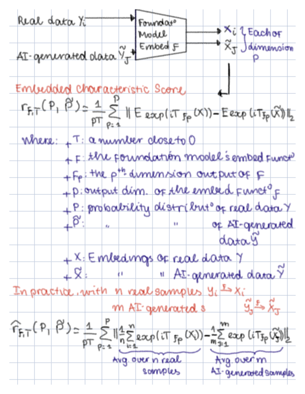
The paper itself introduces the concept of Embedded characteristic score to measure the discrepancies between two distributions of data (real vs. AI-generated).

The paper itself will explain the theoretical rationale behind their choice of how the embeded characteristic score should be defined (that it is a legitimate measure of distance–satisfying the triangle inequality, that its mean approximation converges to the formal definition of expectation, that it is bounded).

Figure 1. Definition of embedded characteristic score.

The paper contains statements for which I am not clear on, and so this blog post is dedicated to helping myself clear up those concepts. Below are the statements I want to understand better:

• When the data distribution is heavy-tailed, the higher moments do not exist or do not converge.
• The values of characteristic function of a distribution is always bounded and always exists.

When the data distribution is heavy-tailed, the higher moments do not exist or do not converge

When a distribution is ‘heavy-tailed’, the probability that the variable $\mathbf{X}$ is far from the mean is higher than , say, that of a normal distribution. The $k-$moment, is defined as $E[\mathbf{X}^k]$, when $X$ has a higher chance to take extreme values, the $k-$moment may not exist because $P(\mathbf{X}^k = \inf) \neq 0$.

In practice, moments of a distribution are estimated through the data: $E[\mathbf{X}^k] \approx \frac{1}{n}\sum_{i=1}^{n}x_i^k$. The same procedure can be repeated mulitple times, obtaining multiple estimates of the $k-$moments of $\mathbf{X}$. When the data is heavy-tailed, we could imagine the sampled $x_i^k$ to take very extreme values, and the estimated $k-$moments may vary greatly across different rounds of sampling. Hence, we can state that the higher moments do not “converge”, i.e. the estimated $k-$moments are unreliable when $k$ is high, and $X$ follows a heavy-tailed distribution.

The values of characteristic functions of a distribution is always bounded and always exists

But first, moment generating functions

Before diving in the concept of chracteristic function, we can revisit the concept of moment generating functions (MGF) to understand why characteristic function is different and necessary. I previously wrote about MGF in a separate blog post, but will outline the key idea here for completeness:

• The MGF of a random variable $X$ is defined as $M_X(t)=E[e^{tX}]$. It is function of $t$.
• Depending on how $X$ is distributed, the MGF may or may not exist. For example, if $X$ is from a normal distribution, the MGF exists and has a very nice analytical form. If $X$ is from a Cauchy distribution, the MGF does not exist.
• MGF is aptly named, because if we take the $k-$th derivative of $M_X(t)$ and plug in $t=0$, we will get $E[X^k]$. This can be proven by first writing the Taylor expansion of $e^{tX} = 1 + \frac{tX}{1!} + \frac{t^2X^2}{2!} + \frac{t^3X^3}{3!} + …$, and then taking the expectation of this with respect to $X$, and plugging in $t=0$.
• When we define a random variable $X$, we (or at least I) tend to think of its PDF function, which specifies $P(X=x)$. The PDF defines an unique distribution. The MGF is an alterative way to define the distribution of $X$, i.e. if two distribution of variables $X$ and $Y$ have the same MGF, then they are identically distributed and also have the same PDF $P(X=x)=P(Y=y)$.
• When we compare two distributions, we can also compare their moments, i.e. checking whether $E[X^k] = E[Y^k]$ for all or many values of $k$. If the moments are equal, then the two distributions for $X$ and $Y$ are identical. This is an alternative approach to comparing the distributions of $X$ and $Y$ based on their PDFs, because theoretically, two variables are identically distributed if and only if they have the same moments.
• A tangent but slightly related note: In a separate scenario, when we have data $x_1, x_2, …, x_n$ from a distribution $X$ parameterized by $\theta$ based on our assumption, we tend to first think of Maximum likelihood estimation to find the optimal value of parameters $\theta$ that would maximize the likelihood of observing $P(x_1,…x_p| \theta)$. A different way to find $\theta$ is to estimate the moments of the variable $X$ based on data, i.e. $\hat{X}^k \approx \frac{1}{n}\sum_{i=1}^{n}x_i^k$ for different values of $k$. Then, if our assumed distribution of $X$ allows us to have a analytical form of the moment generating function, then we can find the optimal values for parameter $\theta$ by fitting the values of analytical formula for $k-$moment ($E(X^k)$ based on the MGF) with the approximated values of $\hat{X}^k$. This approach is called the method of moments, which is just a terminology that scared me for the longest time, just because I dont understand what it is until I do.

As you can see, the moment generating function is very useful, but a limitation of MGF is that it does not always exist, as explained above. Tam and Engelhardt, 2025 (Tam, 2025) paper proposes that instead of comparing the moments of two distributions, we can use a related concept called the characteristic function.

Characteristic function definition

The characteristic function of a random variable $X$ is defined as $\phi_X(t) = E[e^{itX}]$, where $i$ is the imaginary unit. The characteristic function is a function of $t$. Similarly to MGF, the characteristic function is a way to define the distribution of $X$, i.e. if two distribution of variables $X$ and $Y$ have the same characteristic function, then they are identically distributed. This is proven in (Lukacs, 1970).

Why is the characteristic function always bounded?

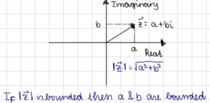
• First, let’s review how a complex number is written in the form of $a+bi$, where $a$ and $b$ are real numbers, and $i$ is the imaginary unit. The magnitude of a complex number $z=a+bi$ is defined as $|z| = \sqrt{a^2+b^2}$.

Figure 2. Imaginary number plane.

• The characteristic function is bounded because $|e^{itX}| = 1$ for any values of $t$ and $X$. This is because: \(\[ \begin{aligned} e^{itX} &= \, (itX)^0 \;+\; \frac{itX}{1!} \;+\; \frac{(itX)^2}{2!} \;+\; \frac{(itX)^3}{3!} \;+\; \cdots && \quad \text{(Taylor expansion of $e^{itX}$)}\\[6pt] &= \,\Bigl(1 \;-\; \frac{t^2X^2}{2!} \;+\; \frac{t^4X^4}{4!} \;-\; \cdots\Bigr) \;+\; i\Bigl(\frac{tX}{1!} \;-\; \frac{t^3X^3}{3!} \;+\; \cdots\Bigr) && \quad \text{}\\[6pt] &= \,\cos(tX) \;+\; i\,\sin(tX) && \quad \text{(Taylor exansion of $\cos$ and $\sin$)}\\[6pt] \end{aligned} \]\)

Hence, $|e^{itX}| = \sqrt{\cos^2(tX) + \sin^2(tX)} = 1$. Therefore, we can always say that the value of $e^{itX}$ lies on the unit circle in the complex plane, and hence the values of the real or complex part of the characteristic function is bounded.

Concluding remarks

• Just like the PDF, the MGF, the characteristic function is another way to define the distribution of a random variable.
• It is always bounded, and hence, it can be used as a more stable measure of the tail behavior of a distribution.
• This is a very primitive treatment of the characteristic function and how it can be used in understanding the behaviors of a distribution. It is my naive attempt to understand this topic. I encourage you to read the paper (Tam, 2025), especially section 3, for a more detailed explanaion of why it is a more stable measurement of the distance between two distributions. Writing this blog made me reread the paper, and I now have a lot more questions than I originally had (such as how the characteristic function is related to the Fourier transform, and more importantly, what exactly is Fourier Transform that I hear a lot about). I will save those for another blog post.

• $Beta(1, N-1)$ converges to $Exponential(\frac{1}{N})$ when $N\rightarrow \infty$.
• Let $Y_{n \cdot d}$ be a matrix of data that is generated such that $Y_{n \cdot d}=X_{n \cdot k} \cdot W_{k \cdot d} + \epsilon_{n \cdot d}$, and each row of $X_{n \cdot k}$, $\mathbf{x_i} \sim N(\mathbf{0}, \sigma_x^2I_{k})$ is drawn from $N(0,1)$, and each row of $\epsilon$, $\epsilon_i\sim N(0, \sigma_{\epsilon}^2I_{d})$. Then, $Y_{n \cdot d}$ is drawn from $N(0,)$.

In general, my first instinct in proving statements about the equivalence between two distributions is to derive the PDF or CDF of the random variable in question. However, I had a hard time proving them through that route this time. Instead, we have to take an alternative approach: Method of moments. Let’s dive in.

The moment of a random variable

If we have a random variable $X$, the $n$-th moment of $X$ is defined as $E[X^n]$. The first moment is the mean, and the second moment is the variance, those are the ones I care to remember, beyond that, we can call them $n$-th moment. In proving that two distributions are equivalent ($Beta(1, N-1)$ and $Exponential(\frac{1}{N})$ in the first opening statement), or that a particular random variable is from a particular distribution $Y\sim Normal(0, \Sigma_{W,\sigma_{\epsilon}, \sigma_{x}})$ in the second opening statement, we can instead show that their moments are equal. If $E[X^n]=E[Y^n]$ for all $n$, then $X$ and $Y$ are identically distributed, or asympotically equally distributed.

Moment generating function

The moment generating function (MGF) of a random variable $X$ is defined as $M_X(t)=E[e^{tX}]$. Here is why MGF takes this particular definition:

• Back in Calculus II (which, imho, is the most omnipresent form of math, backed here), we learned about the Taylor series to estimate the value of a function $f(x)$ for any value of $x$: $f(x)=f(0)+f’(0)x+\frac{f''(0)}{2!}x^2+\cdots$. At the same time, the beauty in $e^x$ function is that its derivative is itself, $e^x$, and $e^{0}=1$ (so when $f(x)=e^x$, $f’(0)= f''(0)= …= 1$). The Taylor series of $e^x$, therefore, is $e^x=1+x+\frac{x^2}{2!}+\frac{x^3}{3!}\cdots$. It’s beautiful!
• Replacing $x$ with $tX$, we get $e^{tX}=1+tX+\frac{(tX)^2}{2!}+\frac{(tX)^3}{3!}\cdots$. Taking the expectation of this with respect to the random variable $X$, we get $M_X(t)=E[e^{tX}]=1+tE[X]+\frac{t^2E[X^2]}{2!}+\frac{t^3E[X^3]}{3!}\cdots$. This is, again, the Taylor expansion of the definition of MGF for random variable $X$, $M_X(t)$.
• The moment generating function is aptly named because if we take the $n-$the derivative of $M_X(t)$ and plug in $t=0$ to the resulting function, we will get $E[X^n]$. For example, $M_X’(0)=E[X]$, $M_X''(0)=E[X^2]$, and so on.
• Not all distributions have a closed-form MGF. However, for most of the distributions that we usually do not avoid, MGF is conveniently written in its Wikipedia page. And if you are ever curious about how the MGF for your distribution of interest is derived but cannot derive it yourself, peek at the solutions manual.

Example of using MGF for a sensible proof

Let’s prove the second opening statement. Here it is in bullet points:

• $\mathbf{Y_{n \cdot d}}$: a matrix of observed data, each row represents a data point, each column corresponds to a feature.
• $n$ is the number of data points, $d$ is the number of features, and $k$ is the number of latent features.
• Generative model assumption: $\mathbf{Y_{n \cdot d}}=\mathbf{X_{n \cdot k}} \cdot \mathbf{W_{k \cdot d}} + \mathbf{\epsilon_{n \cdot d}}$, where $\mathbf{X_{n \cdot k}}$ is the latent feature matrix, $\mathbf{W_{k \cdot d}}$ is the weight matrix (another name is ‘loadings’), and $\epsilon_{n \cdot d}$ represents noise.
  \(\begin{aligned} \begin{pmatrix} \mathbf{y}_1 \\ \mathbf{y}_2 \\ \vdots \\ \mathbf{y}_n \end{pmatrix} = \begin{pmatrix} \mathbf{x}_1 \\ \mathbf{x}_2 \\ \vdots \\ \mathbf{x}_n \end{pmatrix} \cdot \mathbf{W} + \begin{pmatrix} \mathbf{\epsilon}_1 \\ \mathbf{\epsilon}_2 \\ \vdots \\ \mathbf{\epsilon}_n \end{pmatrix} \end{aligned}\)
• Further, we assume that: $\mathbf{x_i} \sim N(\mathbf{0}, \sigma_x^2I_{k})$, and $\mathbf{\epsilon_i} \sim N(\mathbf{0}, \sigma_{\epsilon}^2I_{d})$.
• This, by the way, is the generative model for probabilistic Principal Component Analysis (PPCA), if we have space for another jargon.

The question is: What is the marginal distribution of $\mathbf{Y}$? We can try: $\mathbf{y_i} = \int_{\mathbf{x_i}} \mathbf{x_i}\cdot \mathbf{W}+ \mathbf{\epsilon_i} d{\mathbf{x_i}}$. I was not that good at this maneuver, so instead, we try:

• For the sake of notation simplicity, let’s work through one row of $\mathbf{Y}$ and $\mathbf{X}$ and $\mathbf{\epsilon}$, denoted as $y$ and $x$ $\mathbf{\epsilon}$, respectively, representing one of $N$ independent datapoints. We have $\mathbf{y=x\cdot W + \epsilon}$.
• Now, in a separate scenario for a random $\mathbf{x}$, if $\mathbf{x} \sim Normal(\mathbf{\mu}, \mathbf{\Sigma})$, then $M_{\mathbf{x}}(\mathbf{t}) = exp(\mathbf{t}^T\mathbf{\mu} + \frac{1}{2}\mathbf{t}^T \mathbf{\Sigma} \mathbf{t})$. This is the analytical solution to the MGF of a multivariate normal distribution for $\mathbf{x}$.
• So, when $\mathbf{y=x\cdot W + \epsilon}$, based on the definition of MGF:

Because of the final form of the MGF of $\mathbf{y}$, we can conclude that $\mathbf{y} \sim N(\mathbf{0} , \mathbf{W}^T \sigma_x^2\mathbf{I}_k \mathbf{W}) $.

Extending marginal distribution to inference in PPCA

As mentioned above, our assumption $\mathbf{y=x\cdot W + \epsilon}$ is the generative model for PPCA. In PPCA, we care about infering values of $\mathbf{x}$ and $\mathbf{W}$ given $\mathbf{y}$ as observed data. In theory, based on the above proof, we write the data likelihood $P(\mathbf{y})$ as a function of model parameters $\mathbf{W}, \sigma_x^2, \sigma_{\epsilon}^2$. We can, in theory, take the derivative of the data likelihood with respect to parameters to infer the values of parameters, i.e., setting $\frac{\partial P(\mathbf{Y})}{\partial \mathbf{W}}=\mathbf{0}$ and solve for $\mathbf{W}$. In (Lawrence, 2005), the introduction mentions that ‘PPCA and other latent variables, such as factor analysis or independent component analysis, requires a marginalization of the latent variables and optimization of the parameters’. This turns out to be a lot more challenging, I dont think we can actually find a closed form solution for $\mathbf{W}$ this way (I therefore found what is stated in (Lawrence, 2005) misleading). Instead, we use the Expectation-Maximization (EM) algorithm to iteratively infer the values of $\mathbf{X}$ and $\mathbf{W}, \sigma_x^2, \sigma_{\epsilon}^2$ that maximize the likelihood of the observed data. I know of (Chiu, 2020) that shows an explanation and implementation of the EM algorithm for PPCA, specfically applied to genetics data in which the input matrix only contains ${0,1,2}$.

In a general framework for inference, we observe some data $X$, which we assume to be generated by some latent variables and/or parameters $\theta$, such that we can write down a formula for $P(\mathbf{X}|\theta)$. $theta$ itself is generated from certain distribution, $P(\theta)$. Whether $\theta$ involve some latent variable or parameters, it is usually the goal of our inference to find the distribution or the values of $\theta$ given the observed data $P(\theta|X)$. Example cases of this framework are:

• In a linear regression framework: $y = X\beta + \epsilon$, where $y$ and $X$ are observed. We also assume that $\beta \sim Normal(\mathbf{0}, \sigma^2*\mathbf{I})$.
• In a Variational auto encoder, we assume that our observed data $\mathbf{X}$ of $d$ dimensions is generated, usually through a series of fully connected layers of neural networks $f$, from some latent variables $\mathbf{Z}$, i.e. $\mathbf{X} = f(\mathbf{Z})$. We may also assume that $\mathbf{Z} \sim Normal(\mathbf{0}, \sigma^2*\mathbf{I})$.
• In a Gaussian Mixture Model framework, we observe data $\mathbf{X_i}$’s. We assume that each $X_i$ may be generated from one of the $K$ Gaussian distributions, i.e. $X_i|Z_i=k \sim N(\mu_k, \Sigma_k)$. Here, $Z_i$ is the latent group-indicator variable that we want to infer, $\mu_k$ and $\Sigma_k$ are parameters that we also want to learn. There can be more layers of prior distributions for $Z_i$, $\mu_k$ and $\Sigma_k$, but the backbone of the model model is as indicated above.

Four general approaches to inference

What these models share in common is that it involves observed data $X$ and one or more layers of latent variables $\theta$. What I learned, over the years of connecting the dots (sometimes, very inefficiently, as part of my interdisciplinary training) is that we will almost will always use one of the following approaches for inference (i.e. finding $P(\theta|X)$).

• Can we write down the formula for $P(\theta|X) = \frac{P(\mathbf{X}|\theta)P(\theta)}{\int_{\theta}P(\mathbf{X}|\theta)P(\theta)d\theta}$ into a closed-form formula? If yes then do it and find the value of $\theta$ that maximizes this probability potentially through taking the derivatives $\frac{\partial P(\theta|X)}{\partial \theta}$. This is what is called Maximum A Posterori (MAP) estimation. This case usually happens when we design (assume) $P(\theta)$ to be conjugate prior to the likelihood $P(\mathbf{X}|\theta)$. If you don’t know what conjugate prior is, don’t worry, it won’t be mentioned again in this post.

• If the model is simple enough such that we can clearly break down $\theta$ to latent variables and parameters, then we can potentially use Expectation Maximization (EM) algorithm to find both the expected values of latent variables and the parameters that maximize the likelihood $P(\mathbf{X}|\theta)$ of the observed data. Usually, the first criteria for “simple enough” is that the model has only 1 layer of latent variables, i.e. $\theta \rightarrow \mathbf{X}$ and not $\theta \rightarrow \mathbf{Z} \rightarrow \cdots \rightarrow \mathbf{X}$.
• If the model is such that for each $\theta_i$ as a single latent variable/parameter in $\theta$, we can write down an analytical solution (i.e. usually, a nice known distribution PDF) for $P(\theta_i|X, \theta_{-i})$, then we can use Gibbs sampling to sequentially and repeatedly sample $\theta_i$ from $P(\theta_i|X, \theta_{-i})$ until the values of $\theta_i$’s all converge. This case, again, requires us to analytically explore the closed-form formula for $P(\theta_i|X, \theta_{-i})$ for each $\theta_i$. If you don’t know what Gibbs sampling is, don’t worry, it won’t be mentioned again in this post.
• Lastly, the most versatile approach, in my opinion, is to use Variational Inference. We will zoom into this in the following section.

Note that though the general approaches can act like recipes, our job as practitioners of the discipline is to refine these approaches based on the data at hand, hence requires the arts of implementation, trial and error. Identifying when to use which approach, unfortunately, has to be handled on a case-by-case basis. An important observation is that at each iteration, all of these approaches try to reframe the inference problem into one that can be solved by calculus, i.e. designing a loss function where the model’s latent variables and parameters $\theta$ are variables, taking derivatives, setting to $0$ and solve for $\theta$.

Variational Inference

Let’s try to understand Variational Inference (VI) and where reparameterization trick comes in through a good old example:

• Observed data: $\underbrace{\mathbf{A}}_{N \cdot D}$ and $\underbrace{\mathbf{b}}_{N \cdot 1}$. $N$: sample size, $D$: data dimension.
• Model: $\underbrace{\mathbf{A}}_{N \cdot D} \cdot \underbrace{\mathbf{\beta}}_{D \cdot 1} + \underbrace{\mathbf{\epsilon}}_{N \cdot 1} = \underbrace{\mathbf{b}}_{N \cdot 1}$, where $\mathbf{\beta} \sim Normal(\mathbf{0}, \sigma^2\cdot\mathbf{I_D})$ is the prior distribution that we assume $\mathbf{\beta}$ follows. $\mathbf{\epsilon_i} \sim Normal(\mathbf{0}, \sigma_0^2)$ is the noise term. Assume that $\sigma_0^2$ and $\sigma^2$ are known and fixed.
• Goal: Find $\mathbf{\beta}$ that fit the data, which is usually defined as the $\beta$ that maximize $P(\mathbf{\beta}| \mathbf{A}, \mathbf{b})$.

As mentioned above, there are genrally 4 approaches to this problem and in this case, it can be solved by all 4 approaches. Here, we focus on using Variational Inference (VI).

Step 1: Identifying observed data, latent variables and write down the posterior.

\(\begin{array}{|c|c|c|} \hline & \textbf{General framework} & \textbf{Example} \\ \hline Obs.data & \mathbf{X} & \mathbf{A}, \mathbf{b} \\ Latent & \mathbf{\theta} & \mathbf{\beta} \\ Prior & P(\theta) & P(\beta) = Normal(\mathbf{0}, \sigma^2\cdot\mathbf{I_D}) \\ Likelihood & P(\mathbf{X}\|\theta) & P(\mathbf{A}, \mathbf{b}\|\beta) = P(\mathbf{b}-\mathbf{A}\beta) = Normal(\mathbf{0}, \sigma_0^2) \\ Posterior & P(\mathbf{\theta}\|\mathbf{X}) & P(\beta\|\mathbf{A}, \mathbf{b})=\frac{P(\mathbf{A}, \mathbf{b}\|\beta) P{\mathbf{\beta}}}{\int_{\mathbf{\beta}} P(\mathbf{A}, \mathbf{b}\|\beta) P(\mathbf{\beta}) d\mathbf{\beta}} = Normal(\mathbf{\mu}, \mathbf{\Sigma})\\ \hline \end{array}\)
In the table above, $\mathbf{\mu}$ and $\mathbf{\Sigma}$ has a closed-form solution (due to the fact that we designed both the likelihood and the prior to be Normal). However, most of the time, in the general cases, $P(\mathbf{\theta}|\mathbf{X})$ cannot be derived analysitically. This is when I say to myself: ‘Let's try Variational Inference’.

Step 2: Write down the ELBO for the general case

If this is your first time hearing about the ELBO, just think of it as a fancy word for the loss function for variational inference, which we want to minimize. I have to rederive the ELBO for the general case each time I plan to work with variational inference, just so I can remember what to do next.

Figure 1. Derivation of the ELBO.

Clearly, we want to find $\theta$ that maximizes $P(X)$. What we are saying, in variational inference, is: we cannot find the exact posterior $P(\theta|\mathbf{X})$, and also cannot find the optimal $\theta$ for $P(X)$ since it is not a tractable problem. Instead, we try to generate $\theta$ from a distribution of our design $q(\theta)$ (called the variational distribution), such that we can easily sample from (i.e. some known distributions that we can easily sample by a call to functions in numpy, scipy or pytorch). The distribution $q$ has some parameters (such as mean $\mu$ for a Normal distribution) that we will optimize so that the ELBO is maximized. The ELBO, as shown above, is a lower bound for the log-likelihood $log(P(X))$.

Another amazing advantage of variational infernece is that we potentially ignore the hierarchical dependency between latent variables. If our model is such that $\theta \rightarrow \mathbf{Z} \rightarrow \cdots \rightarrow \mathbf{X}$ where besides $\mathbf{X}$, all other variables are latent and one generates another, then mean-field variational inference allows us to assume that $\theta \sim q_{\theta}$, $Z \sim q_{Z}$, etc., and $q(\text{latent vars.}) = q(\theta)\cdot q(Z) \cdots$. We just have to find the optimal parameters for each $q$ to maximize the ELBO.

Step 3: Write down the ELBO for the case at hand

In the example case, we can choose $q(\mathbf{\beta})$ to be $Normal(\underbrace{\mathbf{\mu}}_{D\cdot 1}, \mathbf{\Sigma})$, where

\(\begin{aligned} \underbrace{\mathbf{\Sigma}}_{D \cdot D}= \begin{bmatrix} \sigma_1^2 & 0 & \cdots & 0 \\ 0 & \sigma_2^2 & \cdots & 0 \\ \vdots & \vdots & \ddots & \vdots \\ 0 & 0 & \cdots & \sigma_D^2 \end{bmatrix} \end{aligned}\)
The parameters for which we will optimize for, therefore, include $\mathbf{\mu}$ and $\sigma_1^2, \sigma_2^2, \cdots, \sigma_D^2$. The ELBO for this case, based on Fig. 1, is:
\(\begin{align} \text{ELBO} &= \mathbb{E}_{q(\mathbf{\beta})} \left[ \log P(\mathbf{A}, \mathbf{b} \mid \mathbf{\beta}) \right] - KL(q(\mathbf{\beta}) \| P(\mathbf{\beta})) \\ &= \sum_{t=1}^{T} \sum_{i=1}^{N} \underbrace{\log P(\mathbf{b}_i - \mathbf{A}_i \mathbf{\beta_t})}_{N(0,\sigma_0^2)} - \underbrace{KL(q(\mathbf{\beta}) \| P(\mathbf{\beta}))}_{KL(N(\mu, \Sigma), N(\mathbf{0}, \sigma^2\cdot \mathbf{I_D}))}\\ \end{align}\)

Step 4: Reparameterize the sampled latent variables from $q$

Note that the parameters for the variational inferences include $\mu$ and $\sigma_1^2, \sigma_2^2, \cdots, \sigma_D^2$. The goal of variational inference, again, is to find the optimal values of these parameters to maximize ELBO. There usually exists an analytical fomular for $KL(q(\mathbf{\beta}) | P(\mathbf{\beta}))$ (which, in our example is the KL divergence between two MultivariateNormal distributions with different means and diagonal covariance matrices). Therefore, we can easily calculate $\frac{\partial KL(q | P)}{\partial \mu_i}$ and $\frac{\partial KL(q | P)}{\partial \sigma_i}$ for each $i \in {1,…D}$. That is one part of $\frac{\partial \text{ELBO}}{\partial \mu_i}$ and $\frac{\partial \text{ELBO}}{\partial \sigma_i}$.

However, due to the fact that we sample $\beta_t \sim N(\mu, \Sigma)$ ($t$ is index of $\beta$ samples) to construct the first part of the ELBO, we cannot easily calculate $\frac{\partial \log P(\mathbf{A}, \mathbf{b} \mid \mathbf{\beta_t}) }{\partial \mu_i}$ and $\frac{\partial \log P(\mathbf{A}, \mathbf{b} \mid \mathbf{\beta_t}) }{\partial \sigma_i}$ for each $i \in {1,…D}$. This is where the reparameterization trick comes in: Instead of directly sample $\beta_t \sim N(\mu, \Sigma)$, we sample $\epsilon_t \sim N(\mathbf{0}, \mathbf{I})$ and calculate $\beta_t = \mu + \Sigma^{1/2} \zeta_t$ where $\zeta_t \sim N(\mathbf{0}, \mathbf{I})$. This way, we can easily calculate $\frac{\partial \log P(\mathbf{A}, \mathbf{b} \mid \mathbf{\beta_t}) }{\partial \mu_i}$ and $\frac{\partial \log P(\mathbf{A}, \mathbf{b} \mid \mathbf{\beta_t}) }{\partial \sigma_i}$ because the randomness in sampling $beta_t$ got attributed to $\zeta_t$, $mu_i$ and $\sigma_i$ are included as an deterministic part of the ELBO.

Step 5: Optimize the ELBO

By this step, we have turned the problem into an optimization problem, and in turn tossing the ball into the court of optimization researchers. We, of course, need to know all the criteria for framing a solvable optimization task (such as making sure all the functions are differentiable, and the loss function should be convex if possible, etc.), but that is a topic for another post. Here, I want to provide a snapshot code for constructing the model for the example case, and the training loop.

import torch
import torch.nn as nn
import torch.optim as optim
import torch.distributions as dist
class model(nn.Module): 
    '''
    The model module specify the generative process to get to the predicted value of b given input A. 
    Required functions: __init__ and forward
    '''
    def __init__(self, D):
        super(model, self).__init__()
        self.D = D
        # set up the parameters for the variational distribution. 
        # use nn.Parameter to declare model parameters, so pytorch can keep track of the gradients
        self.mu = nn.Parameter(torch.zeros(D, 1))  # vector of mu_1, ..., mu_D
        self.sigma = nn.Parameter(torch.ones(D, 1))  # vector of sigma_1, ..., sigma_D

    @staticmethod
    def reparameterize(mu, sigma):
       eps = torch.randn_like(sigma)
       return mu + sigma * eps
    
    def forward(self, A):
        beta = self.reparameterize(self.mu, self.sigma)
        return torch.matmul(A, beta)

#### Generate data ####
N = 1000
D = 2
true_beta = torch.tensor([3, 6]).reshape(D, 1)
A = torch.randn(N, D)
b = torch.matmul(A, true_beta) + torch.randn(N, 1)

#### Loss function ####
def neg_elbo(b_pred, b, model, mu_prior=0, sigma_prior=1):
    epsilon = dist.Normal(1, 1)
    log_llh = epsilon.log_prob(b-b_pred).sum()
    model.eval()
    kl = dist.kl_divergence(dist.Normal(model.mu, model.sigma), dist.Normal(mu_prior, sigma_prior)).sum()
    return -log_llh + kl  # minimize the negative of ELBO

#### Training loop ######
model = model(D)
optimizer = optim.Adam(model.parameters(), lr=0.01)  
# the optimize registers parameters in the model for which it needs to keep track of the gradients
for epoch in range(1000):
    optimizer.zero_grad()
    b_pred = model(A)
    loss = neg_elbo(b_pred, b, model)
    loss.backward()
    optimizer.step()

#### Print the estimated beta ####
print(model.mu, model.sigma)  # model.mu can be used as the estimated beta,
# model.mu and model.sigma combined defines the estimated posterior P(beta|A, b)

Generalizing the model for other cases

So far, I have outlined the steps that I usually take when I try to apply variational inference, with an example in which the variational distribution $q$ is picked to be Normal (and hence, a reparameterization trick for normal distribution). In many cases, due to the nature of the data (categorical, continuous, non-genative, etc.), the choice of the variational distribution $q$ needs to be adapted. For example:

• In the case of Gaussian Mixture Model (presented above, first section), varitational distribution for $Z$, i.e. $q(Z_i)$ should return samples that are one-hot encoded, i.e. $Z_{i}\sim Multinomial(\pi_{q,i})$ so $Z_{i, \text{sampled}} = [0, 0, 1, 0, 0]$ for $K=5$, but the parameters for $q(Z_i)$ should be continuous, i.e. $\pi_{q,i} = [0.1, 0.2, 0.5, 0.1, 0.1]$ for $K=5$. The reparameterization trick should find a way to transform from the continuous parameters $\pi_{q,i}$ to the one-hot encoded $Z_{i, \text{sampled}}$ in a way that $\pi_{q,i}$ is still present in the ELBO. The Gumbel-Softmax trick is one way to do this (Jang, 2016).
• In my recent application, I need the latent varible to be non-negative and continuous, so I picked $q(Z_i) = LogNormal(\mu_i, \sigma_i^2)$. There is, of course, a reparameterization trick for this distribution, $Z_i = \exp(\mu_i + \sigma_i \zeta_i)$ where $\zeta_i \sim N(0, 1)$.

Conclusion

• Usually, when faced with a problem of inference, I usually try to work through four general approaches in increasing levels of problem complexity: MAP estimation, EM algorithm, Gibbs sampling, and Variational Inference.
• Variational inference is usually the most versatile approach, overcoming lots of complications in the hierarchical dependency of latent variables. If we understand the nature of the data requirements, we can pick variational distributions that are both suitable for the data, but also easy to sample from and easy to derive the KL divergence from the prior.
• I always rederive the ELBO for the general case as a separate step in my inference (Fig. 1). It guides me to understand why and what we are doing with varitional inference.
• The reparameterization trick is needed to sample the latent variables $Z$ from variational distribution $q(Z)$, such that the parameters of $q$ are still present in the ELBO, and hence can be optimized. Different variational distributions require different reparameterization tricks, choice of variational inference is dependent on data requirements.

• Uniform distribution $Unif(a,b)$: randomly pick a number between $a$ and $b$.
• Bernoulli distribution $Bern(p)$: flip a coin with probability of head being $p$.
• Binomial distribution $Bin(n,p)$: flip a coin $n$ times, where each time we flip the coin, it tuns up head with probability of $p$.

Beyond these simple distributions, I remembered getting extremely confused about why the rest of the distributions are defined like they are, i.e. how did we come up with the specific form of the $PDF$ functions for these distributions?. Eventually, after seeing them enough, I started to take them as doctrines, to be used and not to be questioned. This post, however, is one of my attempts in breaking that curse. I derive the Beta distribution, linking it to the Dirichlet distribution and eventually reveal how the ideas for this whole post came to be, which is an application of these probability distributions in simulation of sequencing experiments in genomics.

1. Beta distribution and the breaking of a stick

Let’s say I have a stick of length 1, and I want to randomly break it into two pieces. I can do this by randomly picking a number between 0 and 1, $x$ ~ Unif(0,1), and the two lengths of the two pieces will be $x$ and $1-x$. Now, imagine I have to uniformly randomly break the stick into $N$ pieces, where $N$>2 is an integer. How should I do this, i.e. how should I simulate this on the computer?

Here:

import numpy as np
N = 3
us = np.random.uniform(0,1,N-1)  # ex: N=3, us = [0.3,0.6]
us = np.append(us, 0) # ex: us = [0.3,0.6,0]
us = np.append(us, 1)  # ex: us = [0.3,0.6,0,1]
us.sort() # ex: us = [0,0.3,0.6,1]
xs = np.diff(us) # ex: xs = [0.3,0.3,0.4]

Based on the snippet of code above, you can see that we simulate the uniform fragmentation of $1$-length stick by first drawing $N-1$ numbers from the Uniform distribution, sorting them along with $0,1$, and getting their differences.

The question that follows is: What is the probability distribution of the length of one of the $N$ fragments, denoted $X$? The answer, unsurprisingly given the topic of this post, is $\textbf{Beta}$ distribution. In particular, $\mathbf{Beta(1, N-1)}$. Here is why:

• First, the PDF of $X\sim\mathbf{Beta(\alpha, \beta)}$ is given by: $P(X=x) = \frac{x^{\alpha-1}(1-x)^{\beta-1}}{\mathbf{B}(\alpha, \beta)}$, where $\mathbf{B}(\alpha, \beta) = \frac{\Gamma(\alpha)\Gamma(\beta)}{\Gamma(\alpha+\beta)}$ is the Beta function and $\mathbf{G}(\alpha, \beta)$ is the Gamma function, which has its own googlable definition. Therefore, the PDF of $X\sim\mathbf{Beta(1, N-1)}$ is given by: $P(X=x) = \frac{(1-x)^{N-2}}{\mathbf{B}(1, N-1)}$.
• Note that by definitions of the Gamma and Beta functions, we have: \(\begin{align*} \mathbf{B}(1, N-1) &= \frac{\mathbf{\Gamma}(1)\mathbf{\Gamma}(N-1)}{\mathbf{\Gamma}(N)} \\ &= \frac{0!\cdot(N-2)!}{(N-1)!} \\ \end{align*}\)

So, $ \frac{1}{\mathbf{B}(1, N-1)}= N-1 $. Here, Beta function is included in the PDF of the Beta distribution to ensure that $\int_{x=0}^{1}P(\mathbf{X}=x) = 1$.

• Separately, If we denote $\mathbf{Y}$ as the random variable representing the length of one of the $N$ fragments, we just argued above (using the logic of simulation) that $\mathbf{Y}$ can be characterized as the minimum of $N-1$ numbers $\mathbf{u_1, u_2, …, u_{N-1}}$ drawn $i.i.d$ from the Uniform distribution. Now:

• The reason why we used $\propto$ instead of $=$ in the above equations is because in order for $P(\mathbf{Y})$ to be a valid probability distribution, just as in the case for $\mathbf(X)\sim Beta(1, N-1)$, we need $\int_{u=0}^{1}P(\mathbf{Y}=u) = 1$. So we need to find $\mathbf{C}$ such that $\int_{u=0}^{1} \frac{u^0(1-u)^{N-2}}{\mathbf{C}} = 1$. Therefore, $\mathbf{C} = \frac{1}{N-1} = \mathbf{B}(1,N-1)$.
• Overall, we just showed that if $\mathbf{Y}$ is the $\mathbf{r.v}$ of the length of one of the $N$ fragments, then $P(\mathbf{Y}=u)=\frac{u^0(1-u)^{N-2}}{\mathbf{B}(1,N-1)}$, which is the same as the PDF of $\mathbf{X}\sim\mathbf{Beta(1, N-1)} \qquad \blacksquare$.

We can generalize this idea of uniform fragmentation of a $1-$length stick to describe $\mathbf{Beta}(\alpha, \beta)$ as the probability distribution of the $\alpha-$th fragment lengths in ascending order, when we break the stick into $\alpha+\beta$ fragments. Call this variable $\mathbf{Y}_{(\alpha)}$, then:

2. Some extended properties of the Beta distribution:

In uniform fragmentation of the $1-$length stick into $N$ fragments as described above, if $N\rightarrow \infty$, then $\mathbf{Beta}(1, N-1)$ becomes $\mathbf{Exponential}(\frac{1}{N})$ (Tenchov, 1985). I have not been able to fully prove this statement yet, but what I know is possible is that we can prove that when $N\rightarrow \infty$, the first and second moments of the two distributions converge to the same values.

Figure 1. When $N\rightarrow \infty$, the PDF functions of $Beta(1, N-1)$ distribution perfectly overlaps with the PDF function of the $Exponential(1/N)$ distribution.

The Dirichlet distribution is the probability distribution for a vector of $N$ non-negative numbers that sum to $1$, $P(\mathbf{\vec{X}}= (x_1, …x_N))$. Now, if $\mathbf{\vec{X}} \sim \textbf{Dirichlet}(1,1,…,1)$, then we can see the parallel between the marignal distribution of $x_i$, i.e. an individual entry of $\mathbf{\vec{X}}$, will follow $\mathbf{Beta}(1, N-1)$.

3. How the beta distribution and its variants used in genomics?

So far we have walked through the various properties of the Beta distributions, its origins (at least in my mind), and its connection to the other distributions. If you are still curious and have the bandwidth, please read on. If not, you already got the gist of the post.

In genomics, we measure gene expression, epigentic expression through sequencing experiment in which a particular stretch of DNA sequence (let’s call it a transcript without lack of generalizability) is broken into fragments. I was studying about how to properly simulate the result of such an experiment, and an essential step in this pipeline, of course, is to simulate the breaking of a trascript such that each fragment is realistically integers between 200-300 bp in length (which is common in sequencing experiments). There are several ways we can do this:

• Uniform fragmentations: Treat the fragments like a $1-$length stick and break it into $N$ fragments using uniform fragmentation, then multiply the fragments by the total length $L$, and turn the resulting fragment lengths into integers.
• Poission distribution generation: In a lot of bioinformatics applications, Poisson distribution is used because it is a discrete distribution which fits the nature of our data (what else? I don’t know, maybe people also use it out of convenience? but that’s probably too big of an accussation from my part). In this application, we can continually simulate fragment length from a Poission distribution with mean, say, 250bp, until the total length of the fragments is equal to $L$.
• More sophisticated procedures.

What the literature can tell me, based on (Pai AA, 2017) and (Griebel T, 2012), is that the fragment length from a transcript of length $L$, such that the fragment length should be between 200-300 bp, can be simulated using the Weibull distribution with scale $\alpha=200$ and shape $k = log_{10}(L)$. The papers also stated that empirical evidence from doing sequencing experiments, and collecting the data show that this Weibull distribution-based simulation fit the observed fragment length.

Figure 2. The Weibull distribution of fragment length is wildly different from what we get by uniformly breaking the $1-$length strick and multiplying the fragments by the total length $L$.

I was intriqued. How on earth did people come up with using the Weibull distribution for this application in the first place? Or, more likely, how did we invent this distribution in the first place? Unfortunately, I do not have all the answers, but I can show you a few points during my explorations that may justify the choice of the Weibull distribution for this particular application:

One big advantage of modeling the fragment size from the Weibull distribution with scale $\alpha=200$ and shape $k = log_{10}(L)$ is that despite the wide range of possible transcript length $L$ (different gene lengths, and different progress of the transcript down the length of the gene), the distributions of fragment lengths will stay quite similar. This is reflective of what we see in practice: in a sequencing experiment, regardless of the gene length, we would expect to see similar fragment lengths being generated in the experiment.

Figure 3. Each line is showing the PDF of weibull distribution with scale $\alpha=200$ and shape $k = log_{10}(L)$ for varying values of $L$ as the transcript length. The dotted line is showing the mean of the distributions

Finally, if we follow the uniform fragmentation procedure and generate $\mathbf{Y_i} \sim Beta(1, N-1)$, or equivalently $\mathbf{\vec{Y}}=(y_1, … y_N) \sim Dirichlet(1, 1,….,1 )$, and we transform the r.v such that $w_i = y_i^{k}$, where $k= log_{10}(L)$, then the $w_i$ will follow the Weibull distribution with scale $\alpha=1$ and shape $k = log_{10}(L)$. I tried to prove this statement, but I have not succeeded yet, I just know that it is true!

4. Conclusion

• $Beta(\alpha, \beta)$ is the distribution showing the probability of the $\alpha-$th number in ascending order in a pool of $\alpha+\beta$ numbers generated from $Unif(0,1)$.
• $Beta(1, N-1)$ is the distribution of the length of one of the $N$ fragments when breaking a $1-$length stick into $N$ fragments.
• $Beta(1, N-1)$, thererfore, is the marginal distribution of $y_i$ when $\vec{y} \sim Dirichlet(1,1,…,1)$.
• $Beta(1, N-1)$ converges to $Exponential(\frac{1}{N})$ when $N\rightarrow \infty$.
• When we transform $y_i$ from $y_i \sim Beta(1, N-1)$ to $w_i = y_i^{k}$ with $k=log_{10}(L)$ for some number $L$, then the resulting $w_i$ will follow the Weibull distribution with scale $\alpha=1$ and shape $k = log_{10}(L)$.
• Weibull distirbution is used in genomics to simulate the fragment length of a transcript in a sequencing experiment.