In an introduction to probability course, we learned to construct certain probability distributions in very intuitive ways, i.e. we first got introduced to the physical events that gave rise to those distributions and then derived the formulas for the distributions based on first principles. For example:

• Uniform distribution $Unif(a,b)$: randomly pick a number between $a$ and $b$.
• Bernoulli distribution $Bern(p)$: flip a coin with probability of head being $p$.
• Binomial distribution $Bin(n,p)$: flip a coin $n$ times, where each time we flip the coin, it tuns up head with probability of $p$.

Beyond these simple distributions, I remembered getting extremely confused about why the rest of the distributions are defined like they are, i.e. how did we come up with the specific form of the $PDF$ functions for these distributions?. Eventually, after seeing them enough, I started to take them as doctrines, to be used and not to be questioned. This post, however, is one of my attempts in breaking that curse. I derive the Beta distribution, linking it to the Dirichlet distribution and eventually reveal how the ideas for this whole post came to be, which is an application of these probability distributions in simulation of sequencing experiments in genomics.

1. Beta distribution and the breaking of a stick

Let’s say I have a stick of length 1, and I want to randomly break it into two pieces. I can do this by randomly picking a number between 0 and 1, $x$ ~ Unif(0,1), and the two lengths of the two pieces will be $x$ and $1-x$. Now, imagine I have to uniformly randomly break the stick into $N$ pieces, where $N$>2 is an integer. How should I do this, i.e. how should I simulate this on the computer?

Here:

import numpy as np
N = 3
us = np.random.uniform(0,1,N-1)  # ex: N=3, us = [0.3,0.6]
us = np.append(us, 0) # ex: us = [0.3,0.6,0]
us = np.append(us, 1)  # ex: us = [0.3,0.6,0,1]
us.sort() # ex: us = [0,0.3,0.6,1]
xs = np.diff(us) # ex: xs = [0.3,0.3,0.4]

Based on the snippet of code above, you can see that we simulate the uniform fragmentation of $1$-length stick by first drawing $N-1$ numbers from the Uniform distribution, sorting them along with $0,1$, and getting their differences.

The question that follows is: What is the probability distribution of the length of one of the $N$ fragments, denoted $X$? The answer, unsurprisingly given the topic of this post, is $\textbf{Beta}$ distribution. In particular, $\mathbf{Beta(1, N-1)}$. Here is why:

• First, the PDF of $X\sim\mathbf{Beta(\alpha, \beta)}$ is given by: $P(X=x) = \frac{x^{\alpha-1}(1-x)^{\beta-1}}{\mathbf{B}(\alpha, \beta)}$, where $\mathbf{B}(\alpha, \beta) = \frac{\Gamma(\alpha)\Gamma(\beta)}{\Gamma(\alpha+\beta)}$ is the Beta function and $\mathbf{G}(\alpha, \beta)$ is the Gamma function, which has its own googlable definition. Therefore, the PDF of $X\sim\mathbf{Beta(1, N-1)}$ is given by: $P(X=x) = \frac{(1-x)^{N-2}}{\mathbf{B}(1, N-1)}$.
• Note that by definitions of the Gamma and Beta functions, we have: \(\begin{align*} \mathbf{B}(1, N-1) &= \frac{\mathbf{\Gamma}(1)\mathbf{\Gamma}(N-1)}{\mathbf{\Gamma}(N)} \\ &= \frac{0!\cdot(N-2)!}{(N-1)!} \\ \end{align*}\)

So, $ \frac{1}{\mathbf{B}(1, N-1)}= N-1 $. Here, Beta function is included in the PDF of the Beta distribution to ensure that $\int_{x=0}^{1}P(\mathbf{X}=x) = 1$.

• Separately, If we denote $\mathbf{Y}$ as the random variable representing the length of one of the $N$ fragments, we just argued above (using the logic of simulation) that $\mathbf{Y}$ can be characterized as the minimum of $N-1$ numbers $\mathbf{u_1, u_2, …, u_{N-1}}$ drawn $i.i.d$ from the Uniform distribution. Now:

\[\begin{align} P(\mathbf{Y}=u) &\propto P(\min \{u_1, ..., u_{N-1}\} = u) \\ &\propto P(u_{(1)}=u, u_{(2)} >= u, u_{(N-1)}>=u) \\ &\propto P(u_{(1)}=u)P(u_{(2)} >= u)P(u_{(N-1)}>=u) \\ &\propto \frac{1}{1-0}(1-u) \cdots (1-u) \\ &\propto u^0(1-u)^{N-2} \end{align}\]

• The reason why we used $\propto$ instead of $=$ in the above equations is because in order for $P(\mathbf{Y})$ to be a valid probability distribution, just as in the case for $\mathbf(X)\sim Beta(1, N-1)$, we need $\int_{u=0}^{1}P(\mathbf{Y}=u) = 1$. So we need to find $\mathbf{C}$ such that $\int_{u=0}^{1} \frac{u^0(1-u)^{N-2}}{\mathbf{C}} = 1$. Therefore, $\mathbf{C} = \frac{1}{N-1} = \mathbf{B}(1,N-1)$.
• Overall, we just showed that if $\mathbf{Y}$ is the $\mathbf{r.v}$ of the length of one of the $N$ fragments, then $P(\mathbf{Y}=u)=\frac{u^0(1-u)^{N-2}}{\mathbf{B}(1,N-1)}$, which is the same as the PDF of $\mathbf{X}\sim\mathbf{Beta(1, N-1)} \qquad \blacksquare$.

We can generalize this idea of uniform fragmentation of a $1-$length stick to describe $\mathbf{Beta}(\alpha, \beta)$ as the probability distribution of the $\alpha-$th fragment lengths in ascending order, when we break the stick into $\alpha+\beta$ fragments. Call this variable $\mathbf{Y}_{(\alpha)}$, then:

\[\\ P(\mathbf{Y}_{(\alpha)}=u) = \underbrace{\frac{1}{\mathbf{B}(\alpha, \beta)}}_{\text{Normalizing const.}} \cdot \overbrace{u^{\alpha-1}}^{P(\mathbf{Y}_{(1)...(\alpha-1)}<=u)} \cdot \underbrace{\frac{1}{1-0}}_{P(\mathbf{Y}_{(\alpha)}=u)} \cdot \overbrace{(1-u)^{\beta-1}}^{P(\mathbf{Y}_{(\alpha+1)...(\alpha+\beta)}>=u)} \\\]

2. Some extended properties of the Beta distribution:

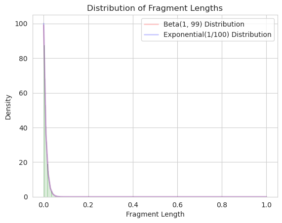
In uniform fragmentation of the $1-$length stick into $N$ fragments as described above, if $N\rightarrow \infty$, then $\mathbf{Beta}(1, N-1)$ becomes $\mathbf{Exponential}(\frac{1}{N})$ (Tenchov, 1985). I have not been able to fully prove this statement yet, but what I know is possible is that we can prove that when $N\rightarrow \infty$, the first and second moments of the two distributions converge to the same values.

The Dirichlet distribution is the probability distribution for a vector of $N$ non-negative numbers that sum to $1$, $P(\mathbf{\vec{X}}= (x_1, …x_N))$. Now, if $\mathbf{\vec{X}} \sim \textbf{Dirichlet}(1,1,…,1)$, then we can see the parallel between the marignal distribution of $x_i$, i.e. an individual entry of $\mathbf{\vec{X}}$, will follow $\mathbf{Beta}(1, N-1)$.

3. How the beta distribution and its variants used in genomics?

So far we have walked through the various properties of the Beta distributions, its origins (at least in my mind), and its connection to the other distributions. If you are still curious and have the bandwidth, please read on. If not, you already got the gist of the post.

In genomics, we measure gene expression, epigentic expression through sequencing experiment in which a particular stretch of DNA sequence (let’s call it a transcript without lack of generalizability) is broken into fragments. I was studying about how to properly simulate the result of such an experiment, and an essential step in this pipeline, of course, is to simulate the breaking of a trascript such that each fragment is realistically integers between 200-300 bp in length (which is common in sequencing experiments). There are several ways we can do this:

• Uniform fragmentations: Treat the fragments like a $1-$length stick and break it into $N$ fragments using uniform fragmentation, then multiply the fragments by the total length $L$, and turn the resulting fragment lengths into integers.
• Poission distribution generation: In a lot of bioinformatics applications, Poisson distribution is used because it is a discrete distribution which fits the nature of our data (what else? I don’t know, maybe people also use it out of convenience? but that’s probably too big of an accussation from my part). In this application, we can continually simulate fragment length from a Poission distribution with mean, say, 250bp, until the total length of the fragments is equal to $L$.
• More sophisticated procedures.

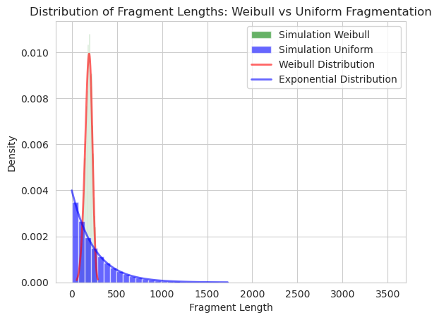
What the literature can tell me, based on (Pai AA, 2017) and (Griebel T, 2012), is that the fragment length from a transcript of length $L$, such that the fragment length should be between 200-300 bp, can be simulated using the Weibull distribution with scale $\alpha=200$ and shape $k = log_{10}(L)$. The papers also stated that empirical evidence from doing sequencing experiments, and collecting the data show that this Weibull distribution-based simulation fit the observed fragment length.

I was intriqued. How on earth did people come up with using the Weibull distribution for this application in the first place? Or, more likely, how did we invent this distribution in the first place? Unfortunately, I do not have all the answers, but I can show you a few points during my explorations that may justify the choice of the Weibull distribution for this particular application:

One big advantage of modeling the fragment size from the Weibull distribution with scale $\alpha=200$ and shape $k = log_{10}(L)$ is that despite the wide range of possible transcript length $L$ (different gene lengths, and different progress of the transcript down the length of the gene), the distributions of fragment lengths will stay quite similar. This is reflective of what we see in practice: in a sequencing experiment, regardless of the gene length, we would expect to see similar fragment lengths being generated in the experiment.

Finally, if we follow the uniform fragmentation procedure and generate $\mathbf{Y_i} \sim Beta(1, N-1)$, or equivalently $\mathbf{\vec{Y}}=(y_1, … y_N) \sim Dirichlet(1, 1,….,1 )$, and we transform the r.v such that $w_i = y_i^{k}$, where $k= log_{10}(L)$, then the $w_i$ will follow the Weibull distribution with scale $\alpha=1$ and shape $k = log_{10}(L)$. I tried to prove this statement, but I have not succeeded yet, I just know that it is true!

4. Conclusion

• $Beta(\alpha, \beta)$ is the distribution showing the probability of the $\alpha-$th number in ascending order in a pool of $\alpha+\beta$ numbers generated from $Unif(0,1)$.
• $Beta(1, N-1)$ is the distribution of the length of one of the $N$ fragments when breaking a $1-$length stick into $N$ fragments.
• $Beta(1, N-1)$, thererfore, is the marginal distribution of $y_i$ when $\vec{y} \sim Dirichlet(1,1,…,1)$.
• $Beta(1, N-1)$ converges to $Exponential(\frac{1}{N})$ when $N\rightarrow \infty$.
• When we transform $y_i$ from $y_i \sim Beta(1, N-1)$ to $w_i = y_i^{k}$ with $k=log_{10}(L)$ for some number $L$, then the resulting $w_i$ will follow the Weibull distribution with scale $\alpha=1$ and shape $k = log_{10}(L)$.
• Weibull distirbution is used in genomics to simulate the fragment length of a transcript in a sequencing experiment.